Architectural synthesis means construction the macroscopic structure of a digital circuit , starting from behavioral model from that can be captured from the #data-flow or #sequence graphs
Circuit Specification for Architectural Synthesis
We capture the behavior of the end circuit via data-flow graphs or sequence graphs spoken about here: Abstract Models. So the rest of this section is going to discuss about resources and constraints and try building intuition over it.
Understanding Resources
In this subsection I try building towards the idea of what resources are. Primarily we can speak about three resources: 1. Functional Resources 2. Memory Resources 3. Interface Resources
- Functional Resources: These are blocks
that process data, they implement arithmetic and logical functions and
can be grouped into two subclasses:
- Primitive Resources: are subcircuits that are ready to use and can be stored in a library, the performance and area parameters of these circuits are characterized and known. Examples of such resources are standard decoders, encoders and arithmetic units.
- Application specific Resources: These are resources that solve some particular subtask and the behavioral model for such circuits cannot be held in the library as above as the functionality is unknown but since we have the sequence graph we can build the model for these when we are parsing them from bottom to top. The implementation of these lower level features can be application specific resources.
- Memory Resources: These are resources that store data - memory arrays, register, register-files etc. Requirements of these resources can be derived from the sequence graph itself, they are also used to transfer data across ports.
- Interface Resources: supports data transfer. Interface resources include busses that may be used as a major means of communication inside a data path. External interface resources are I/O pads and interface circuits.
The major decisions in architectural synthesis are often related to the usage of functional resource. As far as formulating architectural synthesis and optimization problems there is not much difference in between the #functional-resouces and the #application-specific-resources both could be characterized in terms of area and performance and used as building blocks.
If we decide to go via the application-specific-route then we will either need to estimate/predict performance or perform a top-down synthesis to derive area/performance.
So in Dr.Giovanni’s book he points out that there might me resources available for example the notion of ADD, SUB … but the world length of the data might vary so here is when we have the notion of module generators.
When we are synthesizing synchronous circuit which ideally is the case we consider execution time or cycle delay as the time. Some circuit models might only be using a single resource so you will end up only generating the control and this is similar to micro-compilation.
When De Micheli says architectural synthesis reduces to micro-compilation, he means that the hardware design is “finished” (it’s just an ALU), so the only thing left to do is “compile” your algorithm into a list of binary control signals that tell that ALU how to mimic your algorithm step-by-step. It treats the hardware like a tiny, specialized computer and the synthesis tool like a compiler for that computer’s microcode. ## Understanding Constraints
Constraints in architectural synthesis can be classified into two major groups: 1. Interface constraints 2. Implementation constraints
- Interface constraints: Basically how the circuit speaks to the outside world. They can be of certain format or have to adhere to some protocol its not just the type but they might have to obey some timing and bandwidth constraints as well (maintain some data rate).
- Implementation constraints: How the circuit should be internally. Can be area and performance constraints e.g. cycle-time and/or latency bounds. The other can be a binding/resource constraint which basically has to utilize some finite available resources. Architectural synthesis with resources constraint is called as synthesis from partial structure (Read This: https://ieeexplore.ieee.org/document/75629 ) # The Fundamental Architectural Synthesis Problems
We consider not the fundamental problems in architectural synthesis and optimization. We assume that a circuit is specified by: - A sequence graph - A set of functional resources, fully characterized in terms of area and execution delays. - A set of constraints.
For simplicity in this section we can assume the sequence graph to not have any hierarchical graphs and the operations in them are bounded and delays are characterized (Just to get the idea of scheduling and binding). We assume that we have \(n_{\substack{\text{ops}}}\) number of operations and the source and sink are \(v_o\) and \(v_n\) respectively, where \(n = n_{\substack{\text{ops}}} + 1\), Hence the graph \(G_s(V, E)\) has set \(V= \{v_i; i = 1, 2, 3 ..... n\}\) representing the set of operation and \(E = \{(v_i, v_j); i, j = 1, 2, 3 ..... n\}\) representing dependencies.
Architectural synthesis ideally boils down to two stages. First, placing the operations in time and in space, i.e., determining the time interval for their execution and their binding to resources. Second determining the detailed interconnections of the data path and the logic-level specifications of the control unit.
The first stage is just annotating the nodes of the sequence graph with information.
The Temporal Domain: (Aka Scheduling)
For scheduling we will need two attributes for the vertices of the scheduling graph: - The delays of the operations by the set: \[D = \{d_i: i= 1, 2, 3, 4 ...n\}\] - The start time of an operation: \[T= \{t_i; i = 0, 1, 2 .... n\}\]
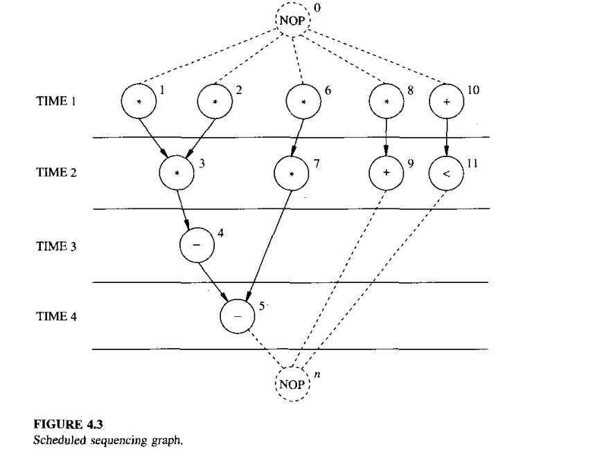
We also assume that the sink and source has zero delay. So put into words, scheduling is the task of determining the start times, subjects to the precedence constraints specified by the sequence graph. The latency of a scheduled sequencing graph is denoted by \(\lambda\) and it is the difference between the start time of the sink and the source.\[\lambda= t_n - t_0\]
A schedule of a sequencing graph is a function \(\psi: V \rightarrow Z^+\) , where \(\psi(v_i)=t_i\) denotes the operation start time such that \(t_i \ge t_j + d_j, \forall i,j: (v_j, v_i) \in E\)
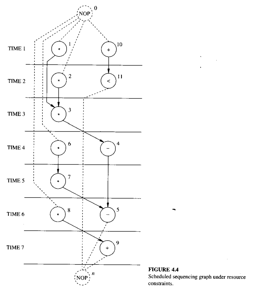
A scheduled sequencing graph is a vertex weighted sequencing graph, where each vertex is labeled by its start time. A schedule may have to satisfy timing and/or resource usage constraints.
 The same graph as above but
with binding constraints might looks something like the below:
The same graph as above but
with binding constraints might looks something like the below:
The Spatial Domain (Aka Binding)
As discussed before we can have various different type of resources so functional resource can be ADD, SUB, MUL … or it can be application specific Boolean function. We can extend the notion of types to functional resources. It is also important to note that a resource type might implement more than one operation for example the resource ALU which performs ADD, SUB, MUL, Comparisons … etc.
We call a resource-type set the set of resources and for simplicity we represent them with enumerations. Thus assuming that there are \(n_{\substack{\text{res}}}\) resource types the set can be defined as: \[\tau: V \rightarrow \{1, 2, 3 ... n_{\substack{\text{res}}}\}\] no-op does not need any binding to any resource, so we just drop the consideration of no-op when binding. It is also important to note that there may be more than one operation with the same type. In this case, resource sharing may be applied or the binding problem can also be extended into a module selection problem (we can have two module doing the same operation example: ripple-carry adder and CLA).
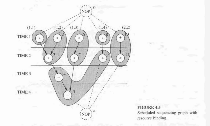
A fundamental concept that relates operations to resources is binding. It specifies which resource implements an operation.
A resource binding is a mapping \(\beta :v \rightarrow R \times z^+\), where \(\beta(v_i) = (t, r)\) denotes that the operation corresponding to \(v_i \in V\), with \(\tau(v_i) = t\), is implemented by the rth instance of resource type \(t \in R\) for each \(i = 1,2,3...., n_{\substack{\text{ops}}}\)
A very simple case of binding is a dedicated resource where every operation is bound to one resource, and the resource binding \(\beta\) is a one-to-one function.
Hierarchical Models
When hierarchical graphs are considered, the concepts of scheduling and binding must be extended accordingly. A hierarchical schedule can be defined by associating a start time to each vertex in each graph entity. The start times are now relative to that of the source vertex in the corresponding graph entity. The start time of the link vertices denote the start time of the source of the linked graph.
To calculate the latency of the graph just parse it bottom-top and you will know the latency and for the model calls just sum the latency of the hierarchy. For branching we can consider the maximum latency of the branching bodies. The delay for iterations is body latency times the maximum number of iterations.
A Hierarchical binding can be defined as the ensemble of bindings of each graph entity, restricted to the operation vertices. Operations in different entities may share resources. While this reduces area and increases performance of the circuit, it complicates the solution of the corresponding binding and resource-constrained scheduling problems. In addition, multiple model calls can be interpreted as viewing multiple shared application specific resource (Refer: Design synthesis under timing constraints).
The Synchronization Problem
There are operations whose delay is unbounded and not known at synthesis time. Scheduling unbounded-latency sequencing graphs cannot be done with traditional techniques. One way to do it is to break the graph into bounded-latency sub-graphs and then scheduling each of these sub-graphs individually.
Area and Performance Estimation
Accurate area and delay estimation is not a simple task. On the other hand architecture design and synthesis requires you to estimate area and performance variations as a result of architectural level decisions.
A schedule provides the latency \(\lambda\) of a circuit for a given cycle-time. A binding provides us with information about the area of a circuit. The following parameters can of-course be easily estimated from a bound sequence graph however to get to this graph we need to some-what accurately estimate these numbers. The estimation is easy when the circuit is resource dominated.
Resource Dominated Circuits
The area and the delay of the resources are known and dominate. The parameters of the other components can be neglected or considered a fixed overhead. Without the loss of generality, assume that the area overhead is zero. The area estimate of a structure is the sum of the areas of the bound resource instances. Equivalently, the total area is the sum of the resource usage. A binding provides the full area but its not needed to estimate one. Since we know the resource bounds we can estimate the schedule as well for a cycle time.
General Circuits
The area estimation is the sum of the areas of the bound resource instances plus the area of the steering logic, registers(or memories), control unit and wiring area. All these components depend on the binding, which in turn depends on the schedule. The latency of the circuit still depends on the schedule, which in turn must take into account the propagation delay of path between register boundaries. Thus performance estimation requires more detailed information. We consider the components of the data path first and then we comment on the control unit.
Registers: All data transferred from a resource to another across a cycle boundary must be stored into some register. An upper bound on the register usage can then be derived by examining ta schedule sequencing graph. This bound is in general loose, because the number of registers can be minimized.
Steering Logic: Steering logic affects the area and the propagation delay. While the area of multiplexers can be easily evaluated, their number requires the knowledge of the binding . Similarly , multiplexers add propagation delays to the resources. Busses can also be used to steer data. In general, circuits may have a fixed number of busses that can support several multiplexed data transfers. So there are couple of delays and area estimation out here: first is the fixed overhead of the busses themselves and the second is the driver and receivers which is nothing but distributed multiplexers.
Wiring: Wiring contributes to the overall area and delay. The wiring area overhead can be estimated from the structure, once a binding is known, by models appropriate for the physical design style of the implementation. The delay is generally proportional to the wire length. So of-course for estimating this we will need the binding structure as well as the
Control Unit: The control circuit contributes to the overall area and delay, because some control signals can be part of the critical path. Consider bounded latency non-hierarchical sequencing graphs. Read only memory based implementations of the control units require an address space wide enough to accommodate all control steps and a word length commensurate tot he number of resources being controlled. Hard-wired control could be done by FSMs.
Strategies for Architectural Optimization
Architecture optimization comprises scheduling and binding Complete architectural optimization is applicable to circuits that can be modeled by sequencing(or equivalent) graphs without a start time or binding annotation. Thus the goal of architectural optimization is to optimize some figure of merit while making sure that we are well within the constraints.
Architectural optimization consists of determining a schedule \(\psi\) and binding \(\beta\) that optimize the objectives (area, latency, cycle-time).
Architectural exploration is often done by exploring the (area/latency) trade-off for different values of the cycle-time. This approach is motivated by the fact that the cycle-time may be constrained to attain one specific value, or some values in an interval, because of system design considerations. Then we can use some scheduling algorithms to explore these trade-offs.
Other important approaches are the search for the (cycle-time/latency) trade-off for some binding or the (area/cycle-time) trade-off for some schedule. These are mostly important when we are scheduling after we are binding and for solving partial problems.
When the circuits are combinational and we have to decide the circuit boundaries to determine cycle time this problem is called retiming.
Data Path Synthesis
Data-path synthesis is a generic term that has often been abused. We distinguish here data-path synthesis techniques at the physical level with those at the architectural level. The former exploit the regularity of data-path structures and are specific to the data-path layout. The latter involve the complete definition of the structural view of the data path. i.e refining the binding information into the specification of all interconnections. To avoid confusion we call this task connectivity synthesis.
There are different methods for data-path synthesis: - bus-oriented - macro-cell-based - array-based
In general the bit-sliced data-paths consume less area and perform better than the others.